Analyzing the genomic and taxonomic composition of an environmental genome using GTDB and sample-specific MAGs with sourmash
C. Titus Brown, Taylor Reiter, and Tessa Pierce Ward
July 2022
Based on a tutorial developed for MBL STAMPS 2022.
You’ll need 5 GB of disk space and 5 GB of RAM in order to run this tutorial. It will take about 30 minutes of compute time to execute all the commands.
In this tutorial, we’ll use sourmash to analyze the composition of a metagenome, both genomically and taxonomically. We’ll also use sourmash to classify some MAGs and integrate them into our analysis.
Install sourmash
First, we need to install the software! We’ll use conda/mamba to do this.
The below command installs sourmash and GNU parallel.
Run:
# create a new environment
mamba create -n smash -y -c conda-forge -c bioconda sourmash parallel
to install the software, and then run
conda activate smash
to activate the conda environment so you can run the software.
Note
Victory conditions: your prompt should start with
(smash)
and you should now be able to run sourmash and have it output usage information!!
Create a working subdirectory
Make a directory named kmers and change into it.
mkdir ~/kmers
cd ~/kmers
Download a database and a taxonomy spreadsheet.
We’re going to start by doing a reference-based compositional analysis of the lemonade metagenome from Taylor Reiter’s STAMPS 2022 tutorial on assembly and binning.
For this purpose, we’re going to need a database of known genomes. We’ll use the GTDB genomic representatives database, containing ~65,000 genomes - that’s because it’s smaller than the full GTDB database (~320,000) or Genbank (~1.3m), and hence faster. But you can download and use those on your own, if you like!
You can find the link to a prepared GTDB RS207 database for k=31 on the the sourmash prepared databases page. Let’s download it to the current directory:
curl -JLO https://osf.io/3a6gn/download
This will create a 1.7 GB file:
ls -lh gtdb-rs207.genomic-reps.dna.k31.zip
and you can examine the contents with sourmash sig summarize:
sourmash sig summarize gtdb-rs207.genomic-reps.dna.k31.zip
which will show you:
>path filetype: ZipFileLinearIndex
>location: /home/stamps2022/kmers/gtdb-rs207.genomic-reps.dna.k31.zip
>is database? yes
>has manifest? yes
>num signatures: 65703
>** examining manifest...
>total hashes: 212454591
>summary of sketches:
>   65703 sketches with DNA, k=31, scaled=1000, abund  212454591 total hashes
There’s a lot of things to digest in this output but the two main ones are:
there are 65,703 genome sketches in this database, for a k-mer size of 31
this database represents 212 billion k-mers (multiply number of hashes by the scaled number)
If you want to read more about what, exactly, sourmash is doing, please see Lightweight compositional analysis of metagenomes with FracMinHash and minimum metagenome covers, Irber et al., 2022.
We also want to download the accompanying taxonomy spreadsheet:
curl -JLO https://osf.io/v3zmg/download
and uncompress it:
gunzip gtdb-rs207.taxonomy.csv.gz
This spreadsheet contains information connecting Genbank genome identifiers to the GTDB taxonomy - take a look:
head -2 gtdb-rs207.taxonomy.csv
will show you:
>ident,superkingdom,phylum,class,order,family,genus,species
>GCF_000566285.1,d__Bacteria,p__Proteobacteria,c__Gammaproteobacteria,o__Enterobacterales,f__Enterobacteriaceae,g__Escherichia,s__Escherichia coli
Let’s index the taxonomy database using SQLite, for faster access later on:
sourmash tax prepare -t gtdb-rs207.taxonomy.csv \
    -o gtdb-rs207.taxonomy.sqldb -F sql
This creates a file gtdb-rs207.taxonomy.sqldb that contains all the information in the CSV file, but which is faster to load than the CSV file.
Download and prepare sample reads
Next, let’s download one of the metagenomes from the assembly and binning tutorial.
We’ll use sample SRR8859675 for today, and you can view sample info here on the ENA.
To download the metagenome from the ENA, run:
wget ftp://ftp.sra.ebi.ac.uk/vol1/fastq/SRR885/005/SRR8859675/SRR8859675_1.fastq.gz
wget ftp://ftp.sra.ebi.ac.uk/vol1/fastq/SRR885/005/SRR8859675/SRR8859675_2.fastq.gz
Now we’re going to prepare the metagenome for use with sourmash by converting it into a signature file containing sketches of the k-mers in the metagenome. This is the step that “shreds” all of the reads into k-mers of size 31, and then does further data reduction by sketching the resulting k-mers.
To build a signature file, we run sourmash sketch dna like so:
sourmash sketch dna -p k=31,abund SRR8859675*.gz \
    -o SRR8859675.sig.gz --name SRR8859675
Here we’re telling sourmash to sketch at k=31, and to track k-mer multiplicity (with ‘abund’). We sketch both metagenome files together into a single signature named SRR8859675 and stored in the file SRR8859675.sig.gz.
When we run this, we should see:
calculated 1 signature for 3452142 sequences taken from 2 files
which tells you how many reads there are in these two files!
If you look at the resulting files,
ls -lh SRR8859675*
you’ll see that the signature file is much smaller (2.5mb) than the metagenome files (~600mb). This is because of the way sourmash uses a reduced representation of the data, and it’s what makes sourmash fast. Please see the paper above for more info!
Also note that the GTDB prepared database we downloaded above was built using the same sourmash sketch dna command, but applied to 65,000 genomes and stored in a zip file.
Find matching genomes with sourmash gather
At last, we have the ingredients we need to analyze the metagenome against GTDB!
the software is installed
the GTDB database is downloaded
the metagenome is downloaded and sketched
Now, we’ll run the sourmash gather command to find matching genomes.
Run gather - this will take ~6 minutes:
sourmash gather SRR8859675.sig.gz gtdb-rs207.genomic-reps.dna.k31.zip --save-matches matches.zip
Here we are saving the matching genome sketches to matches.zip so we can rerun the analysis if we like.
The results will look like this:
overlap     p_query p_match avg_abund
---------   ------- ------- ---------
2.0 Mbp        0.4%   31.8%       1.3    GCF_004138165.1 Candidatus Chloroploc...
1.9 Mbp        0.5%   66.9%       2.1    GCF_900101955.1 Desulfuromonas thioph...
0.6 Mbp        0.3%   23.3%       3.2    GCA_016938795.1 Chromatiaceae bacteri...
0.6 Mbp        0.5%   27.3%       6.6    GCA_016931495.1 Chlorobiaceae bacteri...
...
found 22 matches total;
the recovered matches hit 5.3% of the abundance-weighted query
In this output:
the last column is the name of the matching GTDB genome
the first column is the estimated overlap between the metagenome and that genome, in base pairs (estimated from shared k-mers)
the second column,
p_queryis the percentage of metagenome k-mers (weighted by multiplicity) that match to the genome; this will approximate the percentage of metagenome reads that will map to this genome, if you map.the third column,
p_match, is the percentage of the genome k-mers that are matched by the metagenome; this will approximate the percentage of genome bases that will be covered by mapped reads;the fourth column is the estimated mean abundance of this genome in the metagenome.
The other interesting number is here:
the recovered matches hit 5.3% of the abundance-weighted query
which tells you that you should expect about 5.3% of the metagenome reads to map to these 22 reference genomes.
Note
You can try running gather without abundance weighting:
sourmash gather SRR8859675.sig.gz matches.zip --ignore-abundance
How does the output differ?
The main number that changes bigly is:
the recovered matches hit 2.4% of the query (unweighted)
which represents the proportion of unique kmers in the metagenome that are not found in any genome.
This is (approximately) the following number:
suppose you assembled the entire metagenome perfectly into perfect contigs (note, this is impossible, although you can get close with “unitigs”);
and then matched all the genomes to the contigs;
approximately 2.4% of the bases in the contigs would have genomes that match to them.
Interestingly, this is the only number in this entire tutorial that is essentially impossible to estimate any way other than with k-mers.
This number is also a big underestimate of the “true” number for the metagenome - we’ll explain more later :)
Build a taxonomic summary of the metagenome
We can use these matching genomes to build a taxonomic summary of the metagenome using sourmash tax metagenome like so:
# rerun gather, save the results to a CSV
sourmash gather SRR8859675.sig.gz matches.zip -o SRR8859675.x.gtdb.csv
# use tax metagenome to classify the metagenome
sourmash tax metagenome -g SRR8859675.x.gtdb.csv \
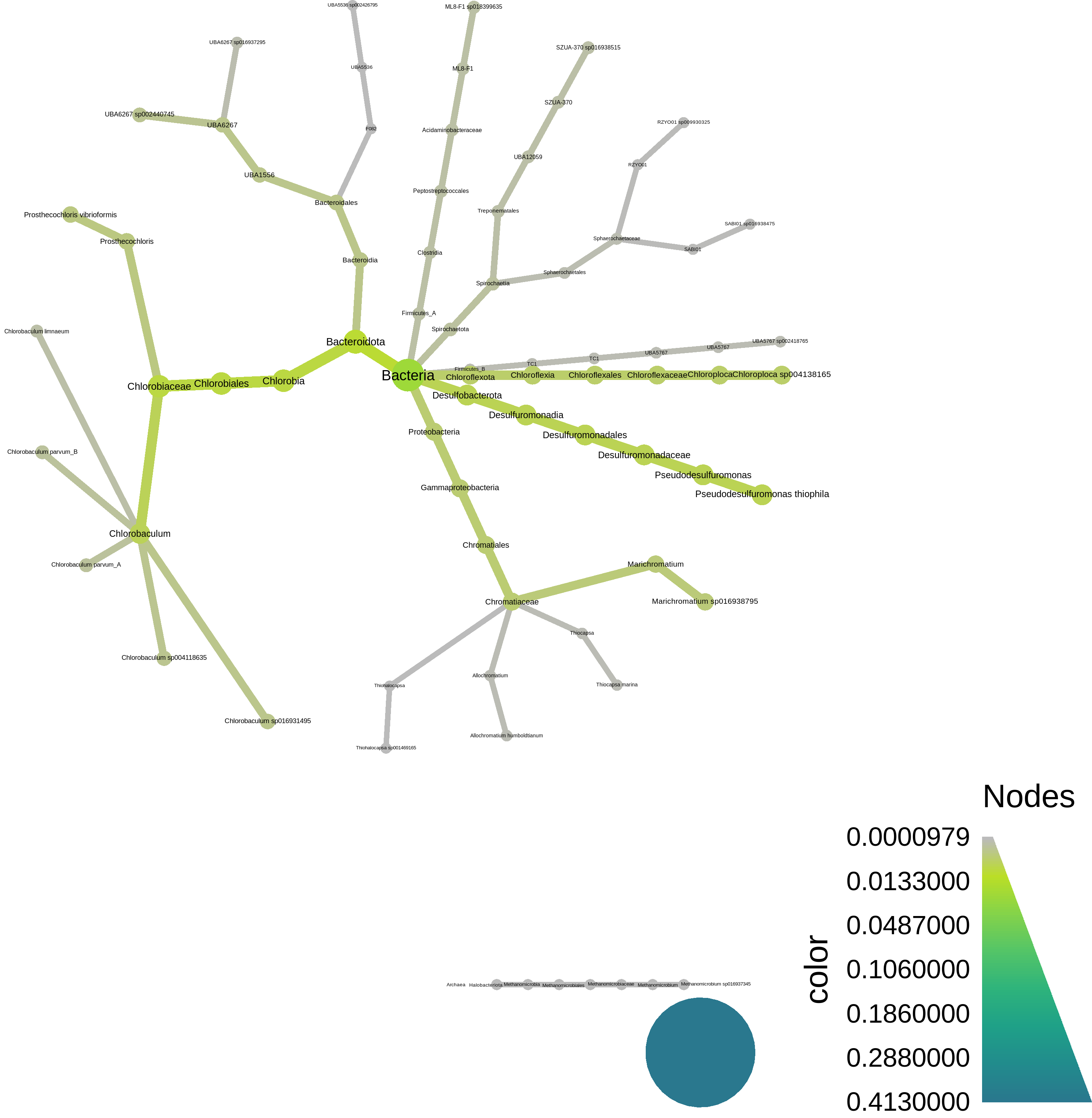
-t gtdb-rs207.taxonomy.sqldb -F human -r order
this shows you the rank, taxonomic lineage, and weighted fraction of the metagenome at the ‘order’ rank.
At the bottom, we have a script to plot the resulting taxonomy using metacoder - here’s what it looks like:
Interlude: why reference-based analyses are problematic for environmental metagenomes
Reference-based metagenome classification is highly dependent on the organisms present in our reference databases. For well-studied environments, such as human-associated microbiomes, your classification percentage is likely to be quite high. In contrast, this is an environmental metagenome, and you can see that we’re estimating only 5.3% of it will map to GTDB reference genomes!
Wow, that’s terrible! Our taxonomic and/or functional analysis will be based on only 1/20th of the data!
What could we do to improve that?? There are two basic options -
(1) Use a more complete reference database, like the entire GTDB, or Genbank. This will only get you so far, unfortunately. (See exercises at end.) (2) Assemble and bin the metagenome to produce new reference genomes!
There are other things you could think about doing here, too, but these are probably the “easiest” options. And what’s super cool is that we did the second one as part of Taylor Reiter’s STAMPS 2022 tutorial on assembly and binning. So can we include that in the analysis??
Yes, yes we can! We can integrate the three MAGs that Taylor generated during her tutorial into the sourmash analysis.
We’ll need to:
download the three genomes;
sketch them with k=31;
re-run sourmash gather with both GTDB and the MAGs.
Let’s do it!!
Update gather with information from MAGs
First, download the MAGs:
# Download 3 MAGs generated by ATLAS
curl -JLO https://osf.io/fejps/download
curl -JLO https://osf.io/jf65t/download
curl -JLO https://osf.io/2a4nk/download
This will produce three files, MAG*.fasta.
Now sketch them:
sourmash sketch dna MAG*.fasta --name-from-first
here, --name-from-first is a convenient way to give them distinguishing names based on the name of the first contig in the FASTA file; you can see the names of the signatures by doing:
sourmash sig describe MAG1.fasta.sig
Now, let’s re-do the metagenome classification with the MAGs:
sourmash gather SRR8859675.sig.gz MAG*.sig matches.zip -o SRR8859675.x.gtdb+MAGS.csv
and look, we classify a lot more!
overlap     p_query p_match avg_abund
---------   ------- ------- ---------
2.3 Mbp       12.1%   99.9%      39.4    MAG2_1
2.2 Mbp       26.5%   99.9%      92.4    MAG3_1
2.0 Mbp        0.4%   31.8%       1.3    GCF_004138165.1 Candidatus Chloroploc...
1.9 Mbp        0.5%   66.9%       2.1    GCF_900101955.1 Desulfuromonas thioph...
1.0 Mbp        2.7%  100.0%      20.3    MAG1_1
0.6 Mbp        0.3%   23.2%       3.1    GCA_016938795.1 Chromatiaceae bacteri...
0.6 Mbp        0.1%   24.5%       2.1    GCA_016931495.1 Chlorobiaceae bacteri...
...
found 24 matches total;
the recovered matches hit 43.5% of the abundance-weighted query
Here we see a few interesting things -
(1) The three MAG matches are all ~100% present in the metagenome. (2) They are all at high abundance in the metagenome, because assembly needs genomes to be ~5x or more in abundance in order to work! (3) Because they’re at high abundance and 100% present, they account for a lot of the metagenome!
What’s the remaining 50%? There are several answers -
(1) most of the constitutent genomes aren’t in the reference database; (2) not everything in the metagenome is high enough coverage to bin into MAGs; (3) not everything in the metagenome is bacterial or archaeal, and we didn’t do viral or eukaryotic binning; (4) some of what’s in the metagenome k-mers may simply be erroneous (although with abundance weighting, this is likely to be a small chunk of things)
Classify the taxonomy of the MAGs; update metagenome classification
Now we can also classify the genomes and update the taxonomic summary of the metagenome!
First, classify the genomes using GTDB; this will use trace overlaps between contigs in the MAGs and GTDB genomes to tentatively identify the entire bin.
for i in MAG*.fasta.sig
do
    # get 'MAG' prefix. => NAME
    NAME=$(basename $i .fasta.sig)
    # search against GTDB
    echo sourmash gather $i gtdb-rs207.genomic-reps.dna.k31.zip \
        --threshold-bp=5000 \
        -o ${NAME}.x.gtdb.csv
done | parallel
(This will take about a minute.)
Here, we’re using a for loop and GNU parallel to classify the three genomes in parallel.
If you scan the results quickly, you’ll see that one MAG has matches in genus Prosthecochloris, another MAG has matches to Chlorobaculum, and one has matches to Candidatus Moranbacteria.
Let’s classify them “officially” using sourmash and an average nucleotide identity threshold of 0.8 -
sourmash tax genome -g MAG*.x.gtdb.csv \
    -t gtdb-rs207.taxonomy.sqldb -F human \
    --ani 0.8
This is an extremely liberal ANI threshold, incidentally; in reality you’d probably want to do something more stringent, as at least one of these is probably a new species.
You should see:
>sample name    proportion   lineage
>-----------    ----------   -------
>MAG3_1             5.3%     d__Bacteria;p__Bacteroidota;c__Chlorobia;o__Chlorobiales;f__Chlorobiaceae;g__Prosthecochloris;s__Prosthecochloris vibrioformis
>MAG2_1             5.0%     d__Bacteria;p__Bacteroidota;c__Chlorobia;o__Chlorobiales;f__Chlorobiaceae;g__Chlorobaculum;s__Chlorobaculum parvum_B
>MAG1_1             1.1%     d__Bacteria;p__Patescibacteria;c__Paceibacteria;o__Moranbacterales;f__UBA1568;g__JAAXTX01;s__JAAXTX01 sp013334245
The proportion here is the fraction of k-mers in the MAG that are annotated.
Now let’s turn this into a lineage spreadsheet:
sourmash tax genome -g MAG*.x.gtdb.csv \
    -t gtdb-rs207.taxonomy.sqldb -F lineage_csv \
    --ani 0.8 -o MAGs
This will produce a file MAGs.lineage.csv; let’s take a look:
cat MAGs.lineage.csv
You should see:
>ident,superkingdom,phylum,class,order,family,genus,species
>MAG1_1,d__Bacteria,p__Patescibacteria,c__Paceibacteria,o__Moranbacterales,f__UBA1
568,g__JAAXTX01,s__JAAXTX01 sp013334245
>MAG2_1,d__Bacteria,p__Bacteroidota,c__Chlorobia,o__Chlorobiales,f__Chlorobiaceae,
g__Chlorobaculum,s__Chlorobaculum parvum_B
>MAG3_1,d__Bacteria,p__Bacteroidota,c__Chlorobia,o__Chlorobiales,f__Chlorobiaceae,
g__Prosthecochloris,s__Prosthecochloris vibrioformis
And if we re-classify the metagenome using the combined information, we see:
sourmash tax metagenome -g SRR8859675.x.gtdb+MAGS.csv \
    -t gtdb-rs207.taxonomy.sqldb MAGs.lineage.csv \
    -F human -r order
Now only 56.5% remains unclassified, which is much better than before!
Interlude: where we are and what we’ve done so far
To recap, we’ve done the following:
analyzed a metagenome’s composition against 65,000 GTDB genomes, using 31-mers;
found that a disappointingly small fraction of the metagenome can be identified this way.
incorporated MAGs built from the metagenome into this analysis, bumping up the classification rate to ~45%;
added taxonomic output to both sets of analyses.
ATLAS only bins bacterial and archaeal genomes, so we wouldn’t expect much in the way of viral or eukaryotic genomes to be binned.
But… how much even assembles?
Let’s pick a few of the matching genomes out from GTDB and evaluate how many of the k-mers from that genome match to the unassembled metagenome, and then how many of them match to the assembled contigs.
First, download the contigs:
curl -JLO https://osf.io/jfuhy/download
this produces a file SRR8859675_contigs.fasta.
Sketch the contigs into a sourmash signature -
sourmash sketch dna SRR8859675_contigs.fasta --name-from-first
Now, extract one of the top gather matches to use as a query; this is “Chromatiaceae bacterium”:
sourmash sig cat matches.zip --include GCA_016938795.1 -o GCA_016938795.sig
Evaluate containment of known genomes in reads vs assembly
Note
If you want to just start here, you can download the files needed for the below sourmash searches from this link.
Now do a containment search of this genome against both the unassembled metagenome and the assembled (but unbinned) contigs -
sourmash search --containment GCA_016938795.sig \
    SRR8859675*.sig* --threshold=0 --ignore-abund
We see:
similarity   match
----------   -----
 23.3%       SRR8859675
  4.7%       SRR8859675_0
where the first match (at 23.3% containment) is to the metagenome. (You’ll note this matches the % in the gather output, too.)
The second match is to the assembled contigs, and it’s 4.7%. That means ~19% of the k-mers that match to this GTDB genome are present in the unassembled metagenome, but are lost during the assembly process.
Why?
Some thoughts and answers
It could be that the GTDB genome is full of errors, and those errors are shared with the metagenome, and assembly is squashing those errors. Yay!
But this is extremely unlikely… This GTDB genome was built and validated entirely independently from this sample…
It’s much more likely (IMO) that one of two things is happening:
(1) this sample is at low abundance in the metagenome, and assembly can only recover parts of it. (2) this sample contains several strain variants of this genome, and assembly is squashing the strain variation, because that’s what assembly does.
Note, you can try the above with another one of the top gather matches and you’ll see it’s entirely lost in the process of assembly -
sourmash sig cat matches.zip --include GCF_004138165.1 -o GCF_004138165.sig
sourmash search --containment GCF_004138165.sig \
    SRR8859675*.sig* \
    --ignore-abund --threshold=0
Summary and concluding thoughts
Above, we demonstrated a reference-based analysis of shotgun metagenome data using sourmash.
We then updated our references using the MAGs produced from assembly and binning tutorial, which increased our classification rate substantially.
Last but not least, we looked at the loss of k-mer information due to metagenome assembly.
All of these results were based on 31-mer overlap and containment - k-mers FTW!
A few points:
We would have gotten slightly different results using k=21 or k=51; more of the metagenome would have been classified with k=21, while the classification results would have been more closely specific to genomes with k=51;
sourmash is a nice one-stop-shop tool for doing this, but you could have gotten similar results by using other tools.
Next steps here could include mapping reads to the genomes we found, and/or doing functional analysis on the matching genes and genomes.